First-order differential equations

Mathematics · First-year university mathematics · about 11 min

A differential equation tells you how a quantity changes rather than giving its value directly. First-order equations involve a first derivative. They model processes such as cooling, growth and changes in concentration. Solving one gives a function whose rate of change follows the stated rule.

The key idea

A separable first-order equation can be written as

\boxed{\frac{dy}{dx}=f(x)g(y)\quad\Longrightarrow\quad\int\frac{1}{g(y)}\,dy=\int f(x)\,dx}

The separation step assumes $g(y)\ne0$ . Check constant solutions with $g(y)=0$ separately.

Draw Cartesian axes with x from 0 to 4 and y from 0 to 4. At every point of the grid x=0,1,2,3,4 and y=0,1,2,3,4 draw one short centred line segment, all of equal projected length, with gradient -0.4(y-2). For y=0 the slope is +0.8; for y=1 it is +0.4; for y=2 it is zero; for y=3 it is -0.4; for y=4 it is -0.8. Draw a dotted horizontal reference line at y=2. No segments have arrowheads, and no solution curve is drawn. — Each short segment shows the local slope specified by the differential equation.

Try it yourself

Change the differential equation and initial point, then follow how the solution curve tracks the slope field.

Separating the variables

For a separable equation, gather terms containing $y$ with $dy$ and terms containing $x$ with $dx$ . Integrate both sides, including a constant of integration. For instance, $dy/dx=2xy$ becomes $dy/y=2x\,dx$ when $y\ne0$ . Integration gives $\ln|y|=x^2+C$ , or $y=Ce^{x^2}$ after allowing the constant to take either sign. Notice that $y=0$ is also a solution. Dividing by $y$ temporarily excludes it, so check for equilibrium solutions before dividing.

Exponential growth and decay

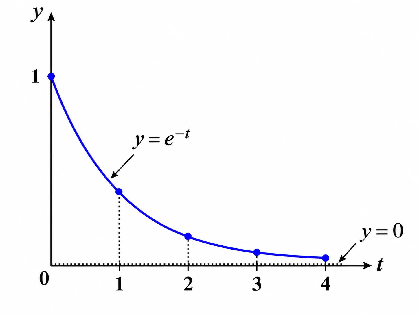
When the rate is proportional to the difference from a fixed level, the model is $dy/dt=-k(y-y_\mathrm{eq})$ with $k>0$ . Its solution is $y(t)=y_\mathrm{eq}+(y_0-y_\mathrm{eq})e^{-kt}$ , where $y_0=y(0)$ . The exponential multiplier decreases over time, so the solution approaches the equilibrium level. A positive sign in $dy/dt=ky$ instead describes growth when $k>0$ . The exponent must be dimensionless: if time is measured in seconds, $k$ has units of inverse seconds.

Draw a graph with horizontal axis t from 0 to 4 and vertical axis y from 0 to 1.2. Plot the smooth function y=e^(-t), starting at the filled point (0,1) and decreasing towards the horizontal axis, with sample guide positions (1,0.3679), (2,0.1353), (3,0.0498), (4,0.0183) determining the curve. Draw a thin horizontal dotted asymptote at y=0, and label the curve y=e^(-t). The curve stays strictly above y=0 for all t shown. — Exponential decay approaches an equilibrium without crossing it in this model.

Initial values and slope fields

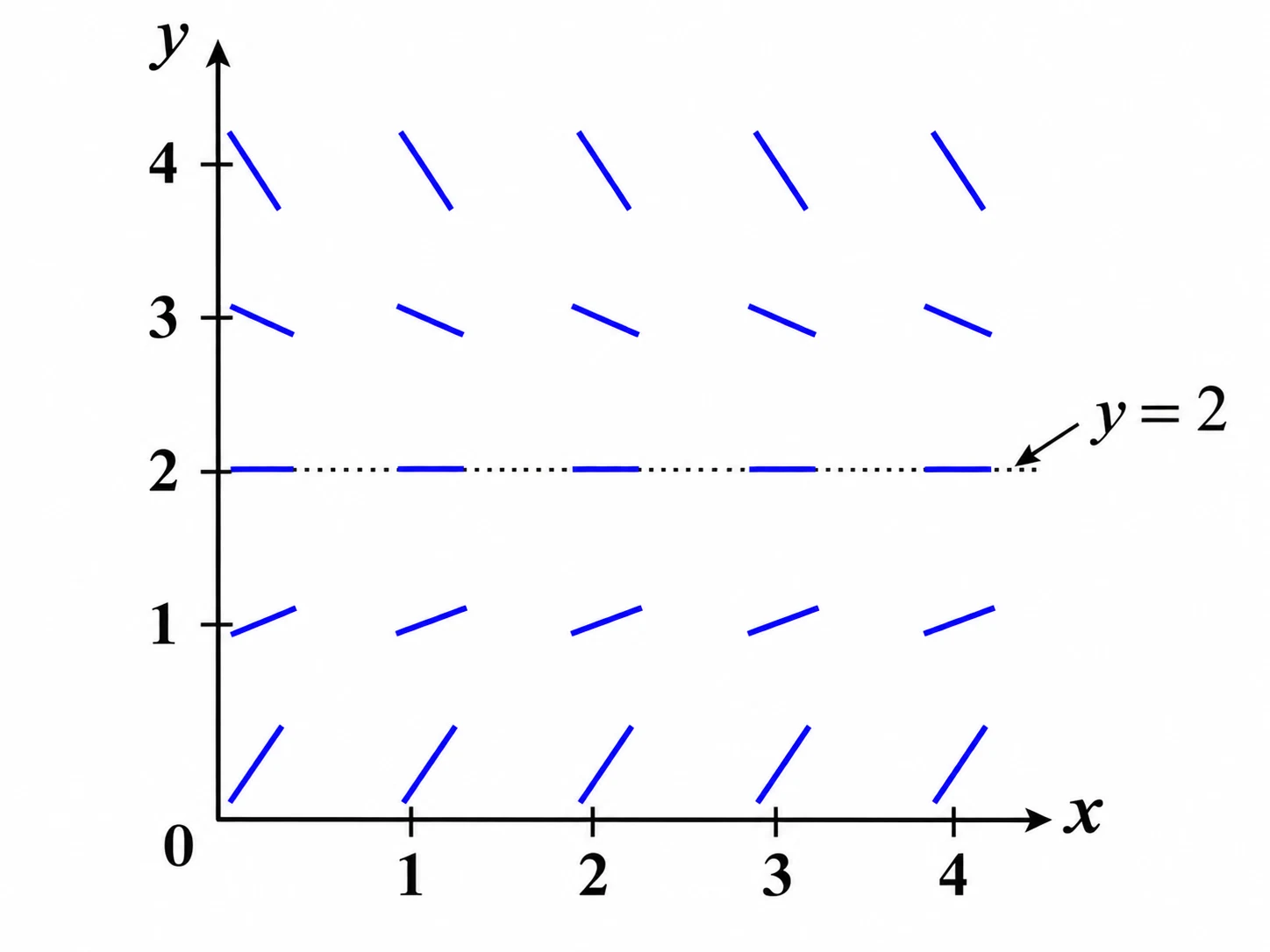
An initial condition such as $y(0)=3$ picks one curve from a family of solutions. Substitute that value after integrating to determine the constant. A slope field gives a visual check: at each point $(x,y)$ , draw a short segment with gradient equal to the right-hand side of the equation. A solution curve follows those local slopes. If the differential equation gives $dy/dx=0$ along a horizontal level, that level can be an equilibrium solution. Check the final expression by differentiating and substituting into the original equation.

Worked example: A cooling object

An object initially at $80\,^\circ\mathrm{C}$ is placed in surroundings at $20\,^\circ\mathrm{C}$ . Its temperature $T$ follows

\frac{dT}{dt}=-0.2(T-20),\qquad T(0)=80,

where $t$ is in seconds and the rate constant is $0.2\,\mathrm{s^{-1}}$ . Find $T(5)$ and the time when $T=30\,^\circ\mathrm{C}$ .

Show the solution

Step 1: Separate and integrate. For $T\ne20$ ,

\frac{dT}{T-20}=-0.2\,dt\quad\Longrightarrow\quad\ln|T-20|=-0.2t+C.

Exponentiating gives $T-20=Ae^{-0.2t}$ .

Step 2: Apply the initial temperature. $80-20=Ae^0$ gives $A=60$ . Hence

T(t)=20+60e^{-0.2t}.

Step 3: Evaluate at $t=5\,\mathrm{s}$ .

T(5)=20+60e^{-1}\approx42.1\,^\circ\mathrm{C}.

Step 4: Find when the temperature reaches $30\,^\circ\mathrm{C}$ .

\begin{aligned}30&=20+60e^{-0.2t}\\\frac16&=e^{-0.2t}\\t&=\frac{\ln6}{0.2}\approx8.96\,\mathrm{s}.\end{aligned}

Answers: $\boldsymbol{T(5)\approx42.1\,^\circ\mathrm{C}}$ and $\boldsymbol{t\approx8.96\,\mathrm{s}}$ .

Common mistakes

Dividing by a function of $y$ without checking when it is zero.

Test constant equilibrium solutions separately before division.

Dropping the integration constant.

Keep an arbitrary constant until the initial condition determines it.

Using a positive exponent for cooling towards equilibrium.

Check that the temperature difference decreases when $k>0$ .

Mixing minutes with a rate given per second.

Use consistent time units so the exponent $kt$ is dimensionless.

Check your understanding

1. If $dy/dx=3x^2$ and $y(0)=2$ , what is $y(x)$ ?

2. Solve $dy/dx=2y$ with $y(0)=3$ .

3. Which constant solution satisfies $dy/dx=x(y-2)$ for every $x$ ?

Still not sure? Talk it through.

Waypoint Mentor's tutor explains this out loud, works through your own problems on a whiteboard, and checks you've got it. Free to start.

Explain this to me