Linear regression and least squares

Statistics · First-year university statistics · about 10 min

When measurements tend to rise or fall together, a straight line can summarise the overall pattern. Linear regression chooses a line that fits the observed points by a specific rule, rather than by eye. The resulting slope, intercept and residuals are useful for describing trends and making predictions, provided the assumptions and limits of the model are understood.

The key idea

The least-squares line and its coefficients are

\hat{y}=b_0+b_1x,\qquad b_1=\frac{\sum_i(x_i-\bar{x})(y_i-\bar{y})}{\sum_i(x_i-\bar{x})^2},\qquad b_0=\bar{y}-b_1\bar{x}.

Here $x$ predicts the response $y$ , $b_1$ is the slope, and $b_0$ is the intercept.

A two-dimensional graph with x-axis rightward and y-axis upward. Plot five small filled dots at coordinates (0,1), (1,2), (2,2), (3,4), (4,5) on axes whose displayed ranges are 0 to 4 horizontally and 0 to 6 vertically. Draw a single straight ascending fitted line passing through the average point (2,2.8), approximately from (0,0.8) to (4,4.8). From the dot at (2,2), draw a vertical dashed segment to the fitted line at (2,2.8) and bracket that segment as a residual e. The line must not pass through all points. No fitted equation or final numerical calculation. — Residuals are the vertical differences between observations and fitted values.

Try it yourself

Move the observed points and inspect how the fitted line and vertical residuals change.

Read the fitted line

Each observed pair $(x_i,y_i)$ has a predictor and a measured response. The fitted value $\hat{y}_i=b_0+b_1x_i$ is what the straight-line model predicts at $x_i$ . The slope $b_1$ is the predicted change in $y$ for a one-unit rise in $x$ ; its units are response units divided by predictor units. The intercept is the predicted response at $x=0$ , although that value may be outside the observed range and may have no useful physical interpretation. Keep the variables in the order stated by the problem. Reversing predictor and response changes the regression.

Least squares and residuals

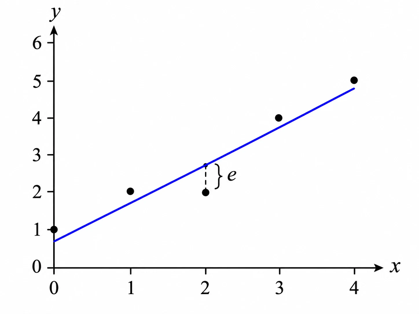
The residual for observation $i$ is $e_i=y_i-\hat{y}_i$ , the vertical distance from a data point to the fitted line. Ordinary least squares chooses the coefficients to minimise $SSE=\sum_i e_i^2$ . Squaring avoids positive and negative residuals cancelling and gives larger errors more weight. For regression with an intercept, the fitted line passes through $(\bar{x},\bar{y})$ . The sums $S_{xx}=\sum(x_i-\bar{x})^2$ and $S_{xy}=\sum(x_i-\bar{x})(y_i-\bar{y})$ provide a compact calculation. If all the $x$ values are identical, $S_{xx}=0$ and a unique slope cannot be obtained.

Predictions and limitations

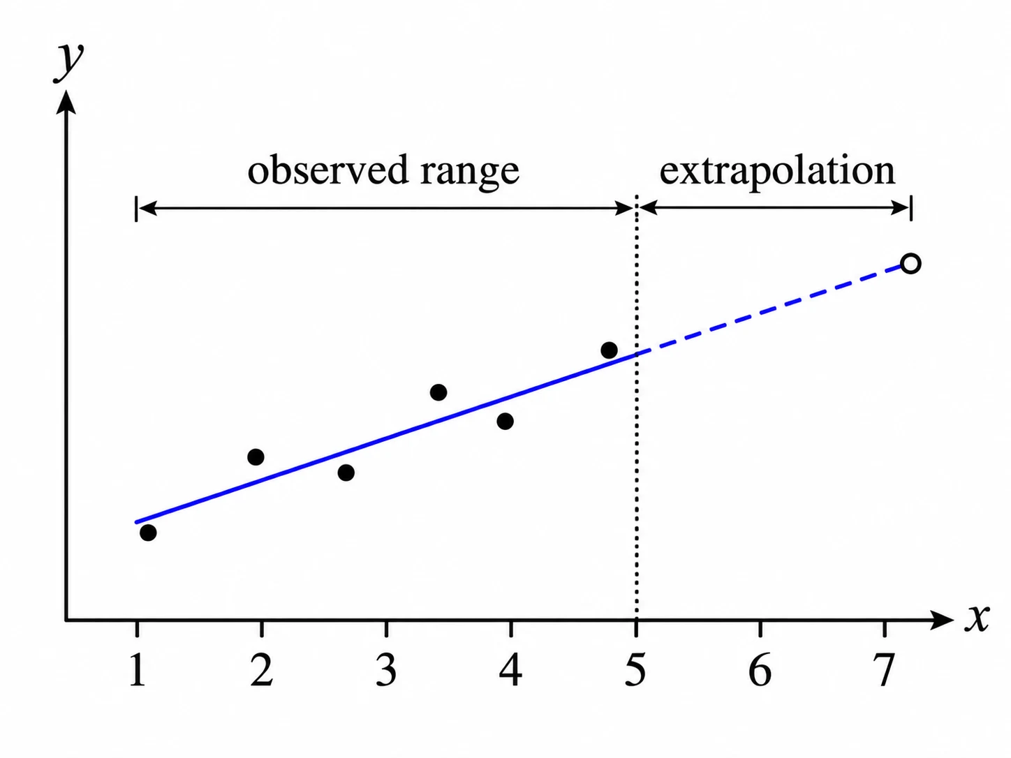
A prediction inside the measured $x$ range is interpolation. A prediction beyond the data is extrapolation and deserves extra caution, even if the fitted line looks convincing. Plot the points and inspect the residuals: a curved pattern suggests a straight line may be unsuitable; a widening spread indicates changing variability. A correlation or a fitted trend does not prove causation. Outliers can strongly affect least-squares coefficients, so do not rely solely on a single calculated slope. Always report the predicted response with its units and distinguish predictions from direct measurements.

Draw Cartesian axes with x horizontal and y vertical. Place six scattered observed points with x between 1 and 5, arranged around a positively sloped straight line. Draw the fitted line solid only within the observed x-range and continue the same line as a dashed extension to x=7. Add a thin vertical dotted boundary at x=5. Place one open circle on the dashed extension at x=7. Indicate the solid segment as interpolation range and the dashed segment as extrapolation. No numeric predictions, slope or intercept. — Beyond the observed predictor range, extending a fitted line is extrapolation.

Worked example: Fitting position measurements over time

A sensor records position $y$ in metres at time $x$ in seconds. The five pairs $(x,y)$ are $(0,1)$ , $(1,2)$ , $(2,2)$ , $(3,4)$ and $(4,5)$ . Fit a least-squares straight line, predict the position at $x=2.5\,\mathrm{s}$ , and calculate the residual for the observation at $x=2\,\mathrm{s}$ .

Show the solution

Calculate the means:

\bar{x}=\frac{0+1+2+3+4}{5}=2\,\mathrm{s},\qquad \bar{y}=\frac{1+2+2+4+5}{5}=2.8\,\mathrm{m}.

Calculate the sums:

S_{xx}=4+1+0+1+4=10\,\mathrm{s^2}.

S_{xy}=3.6+0.8+0+1.2+4.4=10\,\mathrm{m\,s}.

Find slope and intercept:

b_1=\frac{10\,\mathrm{m\,s}}{10\,\mathrm{s^2}}=1\,\mathrm{m/s},\qquad b_0=2.8\,\mathrm{m}-(1\,\mathrm{m/s})(2\,\mathrm{s})=0.8\,\mathrm{m}.

Predict and check a residual: $\hat{y}(2.5\,\mathrm{s})=0.8\,\mathrm{m}+(1\,\mathrm{m/s})(2.5\,\mathrm{s})=3.3\,\mathrm{m}$ . At $x=2\,\mathrm{s}$ , $e=2\,\mathrm{m}-2.8\,\mathrm{m}=-0.8\,\mathrm{m}$ .

Answer: $\hat{y}=0.8\,\mathrm{m}+(1\,\mathrm{m/s})x$ , predicted position $3.3\,\mathrm{m}$ , residual $-0.8\,\mathrm{m}$ .

Common mistakes

Subtracting observed from fitted values when calculating a residual.

Use $e_i=y_i-\hat{y}_i$ , with the observed value first.

Assuming the least-squares line passes through every point.

It minimises the sum of squared residuals; individual residuals are usually non-zero.

Giving a slope without its units.

Divide the response units by the predictor units.

Treating extrapolated predictions or correlation as proof of a physical cause.

Check the data range, alternative explanations and the residual pattern.

Check your understanding

1. A fitted line is $\hat{y}=1+2x$ . What does it predict at $x=3$ ?

2. At one data point the measured response is $9$ and the fitted response is $7$ . What is the residual?

3. What quantity does ordinary least squares minimise for a line fitted with vertical residuals?

Still not sure? Talk it through.

Waypoint Mentor's tutor explains this out loud, works through your own problems on a whiteboard, and checks you've got it. Free to start.

Explain this to me