Price elasticity of demand

Economics · Senior school economics · about 10 min

A price change rarely produces the same quantity response for every product. Price elasticity of demand measures that responsiveness in percentage terms so goods with different prices and quantities can be compared. It also helps explain whether a price rise is likely to increase or decrease sellers' total revenue.

The key idea

For two observed price and quantity combinations, use midpoint elasticity:

E_d=\frac{(Q_2-Q_1)/[(Q_1+Q_2)/2]}{(P_2-P_1)/[(P_1+P_2)/2]}

Here $P$ is price and $Q$ is quantity demanded. A normal downward-sloping demand curve gives a negative signed elasticity.

Draw axes with Q horizontal and P vertical. From one shared middle point draw two straight downward-sloping demand lines: a relatively flat one labelled elastic and a relatively steep one labelled inelastic. Add two thin horizontal guide lines marking the same initial and higher price level. Show the horizontal spans between the intersections of each demand curve with these two price lines; the flat line must have the larger change in quantity. Do not show numerical values, computed elasticity or revenue. — Flatter demand produces a larger quantity response to the same price movement.

Interpret the magnitude

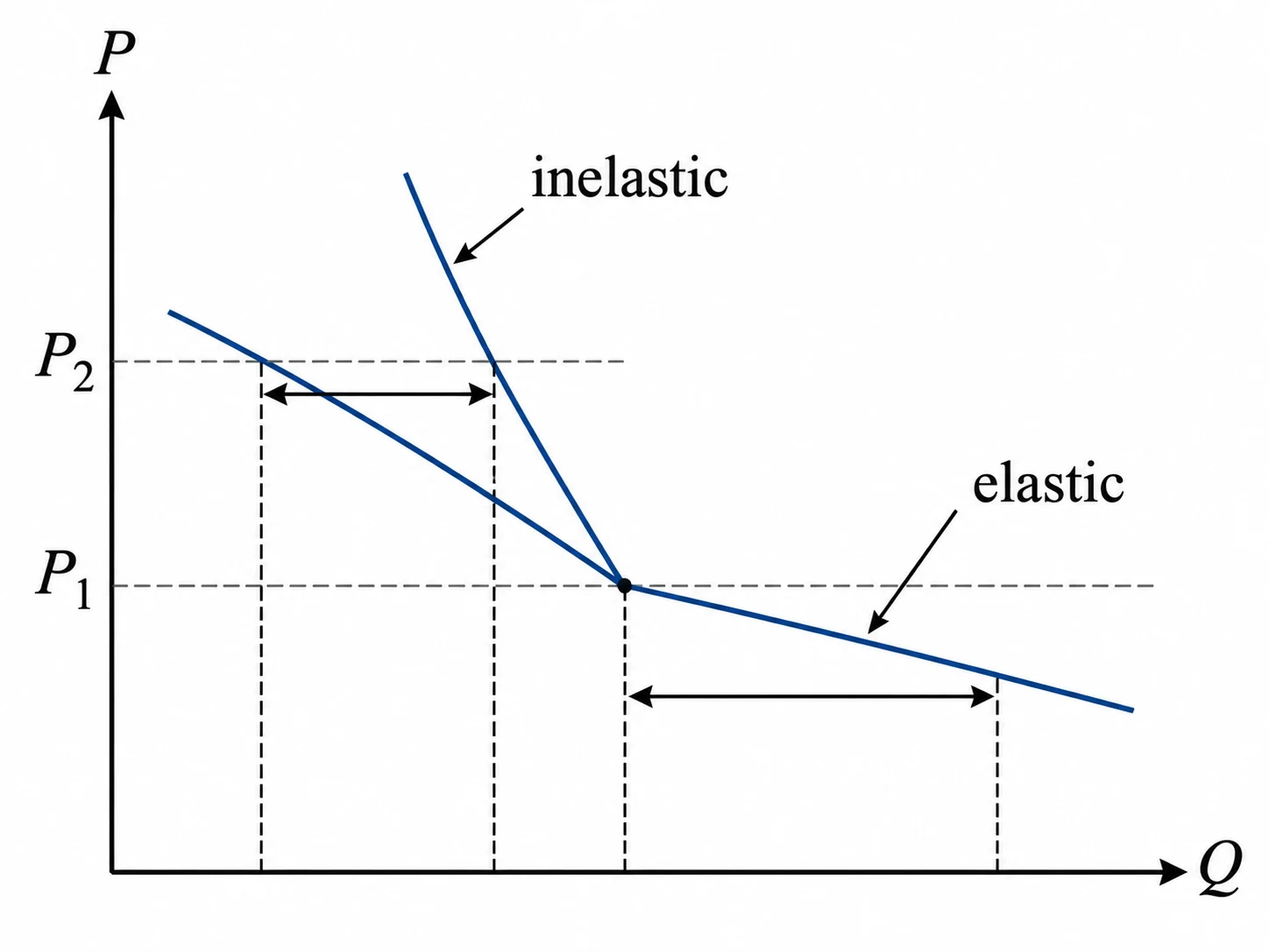
Economists often classify demand by the absolute value $|E_d|$ . If it exceeds one, demand is elastic: quantity changes by a larger percentage than price. If it is below one, demand is inelastic. At exactly one, it is unit elastic. The minus sign usually reflects the inverse relation between price and quantity and is not itself a measure of strength. Elasticity is unit-free because it compares percentages. Demand may be more elastic when close substitutes exist or buyers have more time to adjust their choices.

Why use the midpoint method

A conventional percentage change based only on the starting value produces different elasticity estimates for a rise and the equal reverse fall. The midpoint method uses the average of the two prices and the average of the two quantities, making the measured magnitude the same in either direction. Mark the two price-quantity points before calculating so the changes have consistent signs. For a tiny change at one point of a differentiable demand curve, point elasticity is $E_d=(dQ/dP)(P/Q)$ ; this is different from an arc elasticity over a finite interval.

Elasticity and total revenue

Total revenue is $TR=PQ$ . With elastic demand, a small price rise generally reduces revenue because the percentage fall in quantity is larger. With inelastic demand, a small price rise generally raises revenue. Under unit elasticity, total revenue is locally unchanged for a small price change. For larger finite changes, calculate the initial and final $PQ$ values rather than relying only on the elasticity category. These statements concern revenue, not profit, because costs have not been considered.

Worked example: Price change for a weekly product

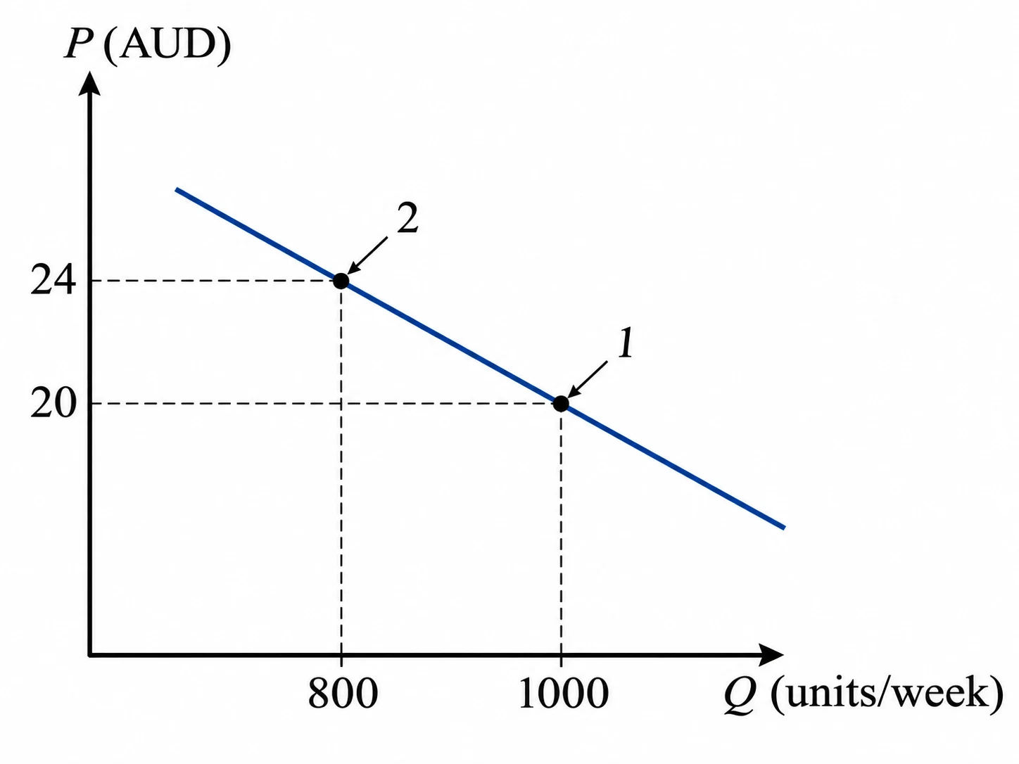
A seller raises a product's price from $20\,\mathrm{AUD}$ to $24\,\mathrm{AUD}$ per unit. Weekly quantity demanded falls from $1\,000$ to $800$ units. Find the midpoint price elasticity of demand, classify it and calculate the change in weekly total revenue.

Draw a simple downward-sloping linear demand curve on axes with quantity Q on the horizontal and price P on the vertical. Mark point 1 at (Q=1000,P=20) and point 2 at (Q=800,P=24), with point 2 visibly above and to the left of point 1. Draw thin horizontal and vertical dashed projection guides from both points to axes. Put 800 and 1000 on Q axis and 20 and 24 on P axis, spaced in correct proportions. No elasticity, total revenue or answer is printed. — The midpoint calculation compares percentage changes between two observations.

Show the solution

Compute midpoint percentage changes:

\frac{\Delta Q}{Q_{\mathrm{avg}}}=\frac{800-1\,000}{(1\,000+800)/2}=\frac{-200}{900}\approx-0.22222

\frac{\Delta P}{P_{\mathrm{avg}}}=\frac{24-20}{(20+24)/2}=\frac{4}{22}\approx0.18182

Divide the changes:

E_d=\frac{-200/900}{4/22}=-\frac{11}{9}\approx-1.22

Since $|E_d|>1$ , demand is elastic over this interval.

Compare weekly revenue:

TR_1=20(1\,000)=20\,000\,\mathrm{AUD}

TR_2=24(800)=19\,200\,\mathrm{AUD}

\Delta TR=19\,200-20\,000=-800\,\mathrm{AUD}

Answer: midpoint elasticity is approximately $-1.22$ (elastic), and weekly revenue decreases by $800\,\mathrm{AUD}$ , or $4\%$ .

Common mistakes

Using different percentage-change bases

For an arc over two points, divide both changes by their respective midpoints.

Calling a negative number less than one inelastic

Use the magnitude $|E_d|$ when classifying demand.

Reversing price and quantity changes

Put percentage quantity change in the numerator and percentage price change in the denominator.

Treating revenue and profit as identical

Calculate revenue as price times quantity; profit also requires costs.

Check your understanding

1. Price increases from $10$ to $12$ , while quantity demanded falls from $100$ to $80$ . What is midpoint $E_d$ (approximately)?

2. If demand is inelastic with $|E_d|=0.4$ , what usually happens to total revenue after a small price rise, all else equal?

3. What does $E_d=0$ mean?

Still not sure? Talk it through.

Waypoint Mentor's tutor explains this out loud, works through your own problems on a whiteboard, and checks you've got it. Free to start.

Explain this to me