Taylor series

Mathematics · First-year university maths · about 10 min

A complicated smooth function can often be approximated near a chosen point by a polynomial. Taylor polynomials use the function and its derivatives at that point to construct successively better local approximations. This is useful for evaluating functions numerically, simplifying models and estimating how accurate a short approximation will be.

The key idea

The Taylor polynomial of degree $n$ about $x=a$ is

P_n(x)=\sum_{k=0}^{n}\frac{f^{(k)}(a)}{k!}(x-a)^k.

Here $f^{(k)}(a)$ is the $k$ th derivative at $a$ (with $f^{(0)}=f$ ), and $k!$ is the factorial.

Draw x and y coordinate axes with horizontal x from -1.5 to 1.5 and vertical y from -1 to 5. Draw the smooth curve y=exp(x), passing through (0,1), and three distinct comparison curves P1(x)=1+x, P2(x)=1+x+x^2/2, P3(x)=1+x+x^2/2+x^3/6. Use different line patterns, not multiple colours: solid exp, long-dashed P1, dotted P2, short-dashed P3. All curves meet at (0,1); the higher-order approximations track the solid curve more closely near x=0. Attach each label adjacent to its curve where distinguishable, not on top of another. — Higher-degree Maclaurin polynomials follow the exponential curve more closely near zero.

Try it yourself

Increase the polynomial degree and inspect where it begins to match the original curve.

Build the polynomial

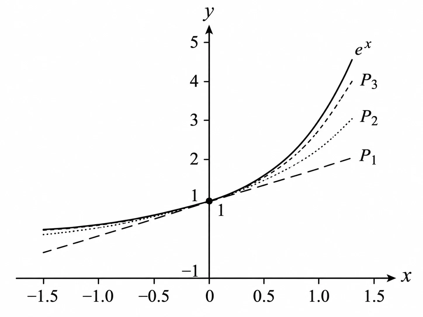
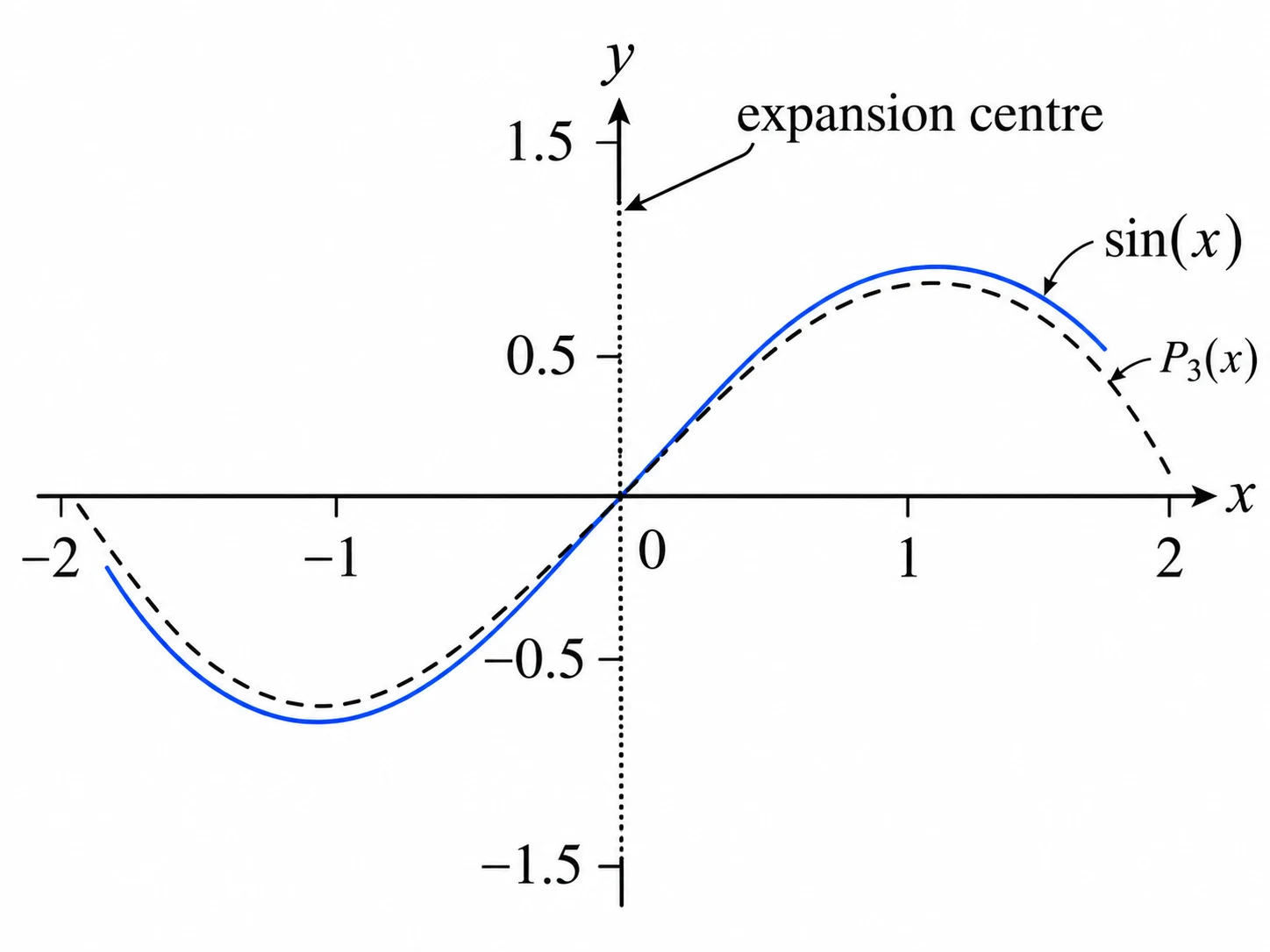
Start with the function value $f(a)$ , add the linear term $f'(a)(x-a)$ , then add terms using higher derivatives divided by their factorials. When $a=0$ , the polynomial is called a Maclaurin polynomial. For example, all derivatives of $e^x$ equal $e^x$ , so at $a=0$ every derivative has value $1$ . The degree-three approximation is $P_3(x)=1+x+x^2/2+x^3/6$ . For $\sin x$ , the even-power coefficients vanish at zero and the first terms are $x-x^3/6+x^5/120$ . Match the requested polynomial degree, not the number of non-zero terms.

Approximate near the centre

Evaluate the polynomial at a nearby $x$ in place of the original function. Keeping extra terms often improves accuracy close to the expansion centre, although the rate depends on the function and the interval. For example, the quadratic Maclaurin approximation $1+x+x^2/2$ tracks $e^x$ well when $|x|$ is small. The approximation is local: a polynomial that works near $a$ need not remain accurate far away. State the expansion centre, the highest retained power, and the numerical answer at the precision requested by the question.

Bound the omitted terms

The error is $R_n(x)=f(x)-P_n(x)$ . If the $(n+1)$ th derivative has absolute value at most $M$ between $a$ and $x$ , Taylor's remainder bound gives $|R_n(x)|\le M|x-a|^{n+1}/(n+1)!$ . This provides a defensible accuracy estimate without knowing the exact answer. Find $M$ over the whole relevant interval, not only at $a$ . A Taylor series may represent the original function only within a certain domain, so a formal infinite series must not be assumed valid at every possible $x$ . For exams, check whether the question asks for a polynomial approximation or a convergent series.

Draw axes with x horizontal from -2 to 2 and y vertical from -1.5 to 1.5. Show a solid smooth curve y=sin(x) and a dashed cubic curve y=x-x^3/6. Both curves cross the origin with identical slope and remain close near x=0; they separate near x=-2 and x=2. Add a thin vertical dotted guide at x=0 marked expansion centre, and use separate line-style labels near the right of the curves. Do not write numeric error estimates. — A polynomial approximation is most reliable near the point where it was built.

Worked example: Approximate an exponential

Use the degree-three Maclaurin polynomial for $e^x$ to approximate $e^{0.2}$ . Compare with the numerical value of $e^{0.2}$ and give a Lagrange error bound over $0\le x\le0.2$ .

Show the solution

Derivatives at zero: For $f(x)=e^x$ , each derivative at $0$ equals $1$ .
Degree-three polynomial:

P_3(x)=1+x+\frac{x^2}{2}+\frac{x^3}{6}.

Evaluate at $x=0.2$ :

P_3(0.2)=1+0.2+\frac{0.2^2}{2}+\frac{0.2^3}{6}=1.2213333\ldots

Check the actual error: $e^{0.2}\approx1.2214028$ , so $|e^{0.2}-P_3(0.2)|\approx0.0000694$ .
Bound the remainder: Since $f^{(4)}(x)=e^x\le e^{0.2}$ on this interval,

|R_3(0.2)|\le\frac{e^{0.2}(0.2)^4}{4!}\approx0.00008143.

Answer: $e^{0.2}\approx1.2213333$ using $P_3$ , with actual error about $0.0000694$ and rounded upper bound $0.00008143$ .

Common mistakes

Leaving out the factorial under a derivative coefficient.

The coefficient of $(x-a)^k$ is $f^{(k)}(a)/k!$ .

Confusing degree with the number of displayed non-zero terms.

A degree-five polynomial can omit powers whose derivatives vanish at the centre.

Assuming a local approximation is equally accurate far from its centre.

Inspect $|x-a|$ and use a remainder bound or compare higher degrees.

Using the derivative at the centre alone as a global remainder bound.

Bound the next derivative on the entire interval between the centre and the evaluation point.

Check your understanding

1. Which is the degree-four Maclaurin polynomial of $\cos x$ ?

2. Using $P_2(x)=1+x+x^2/2$ for $e^x$ , what is $P_2(0.1)$ ?

3. What is the coefficient of $x^3$ in the Maclaurin series for $\sin x$ ?

Still not sure? Talk it through.

Waypoint Mentor's tutor explains this out loud, works through your own problems on a whiteboard, and checks you've got it. Free to start.

Explain this to me